Mixture model
A Gaussian mixture model is a probabilistic way of representing subpopulations within an overall population. We only observe the data, not the subpopulation from which observation belongs.
We have $N$ random variables observed, each distributed according to a mixture of K gaussian components. Each gaussian has its own parameters, and we should be able to estimate the category using Expectation Maximization, as we are using a latent variables model.
Now, in a bayesian scenario, each parameter of each gaussian is also a random variable, as well as the mixture weights. To estimate the distributions we use Variational Inference, which can be seen as a generalization of the EM algorithm. Be sure to check this book to learn all the theory behind gaussian mixtures and variational inference.
Here is my implementation for Variational Gaussian Mixture Model.
#Variational Gaussian Mixture Model


#Constant for Dirichlet Distribution
dirConstant <- function(alpha){
  res <- 1
  for(i in 1:length(alpha)){
    res <- res * gamma(alpha[i])
  }
  return(gamma(sum(alpha))/res)
}


BWishart <- function(W, v){
  D <- ncol(W)
  elem1 <- (det(W))^(-v/2)
  elem2 <- (2^(v*D/2)) * (pi^(D*(D-1)/4))
  elem3 <- 1
  for(i in 1:D){
    elem3 <- elem3 * gamma((v+1-i)/2)
  }
  return(elem1 / (elem2 * elem3))
}

#Log precision expected value
espLnPres <- function(W, v){
  res <- 0
  D <- ncol(W)
  for(i in 1:D){
    res <- res + digamma((v+1-i)/2)
  }
  res <- res + D*log(2) + log(det(W))
  return(res)
}

#Wishart distribution entropy
entropyWishart <- function(W, v){
  D <- ncol(W)
  return(-log(BWishart(W,v)) - ((v-D-1)/2) * espLnPres(W,v) + (v*D)/2)
}

# Estimating mixture parameters

vgmm <- function(X, K, iter = 100, eps = 0.001){
  D <- ncol(X)
  N <- nrow(X)

  #Hyperparameters initialization
  m0 <- rep(0, D)  # mean
  W0 <- diag(D)  # precision
  v0 <- D  # degrees of freedom:  n > p-1
  alpha0 <- 1/K # Dirichlet parameter
  beta0 <- 1  # Variance for mean

  #For each category
  #Initialize the means with centroids from k-means
  mk <- kmeans(X,K)$centers

  #Initialize presicions with diagonal  matrix
  Wk <- array(0, c(D, D, K))

  for(i in 1:K)
    Wk[,,i] <- W0

  vk <- rep(v0, K)

  #Initialize hyperparameters
  betak <- rep(beta0, K)
  alphak <- rep(alpha0,K)

  # Necessary terms for calculate responsabilities
  ln_pres <- rep(0,K)
  ln_pi <- rep(0,K)
  E_mu_pres <- matrix(0, N, K)


  # Iterate

  for(it in 1:iter){

    #Responsabilities
    r <- matrix(0,N, K)

    #####################  Variational E-Step  ##########################33

    for(i in 1:K){

      #Log precision
      ln_pres[i] <- 0

      for(j in 1:D){
        ln_pres[i] <- ln_pres[i] + digamma((vk[i] + 1 - j) /2)
      }

      ln_pres[i] <- ln_pres[i] + D * log(2) + log(det(Wk[,,i]))

      alpha <- sum(alphak)

      ln_pi[i] <- digamma(alphak[i]) - digamma(alpha)

      #E[mu,pres] (expected value of joint distribution of mu and pres)
      for(k in 1:N){
        E_mu_pres[k,i] <- (D / betak[i]) + vk[i] * t(X[k,] - mk[i,]) %*%
          Wk[,,i] %*% (X[k,] - mk[i,])  #10.64

        r[k,i] <- ln_pi[i] + 0.5 * ln_pres[i] - (D/2) *log(2*pi) -
          0.5 * E_mu_pres[k,i]

      }
    }

    # Exp-log-sum trick for numerical stability
    rho <- apply(r, 1, function(x){
      offset <- max(x)
      y <- x - offset
      return(exp(y)/sum(exp(y)))
    })

    rho <- t(rho)

    ########################### Variational M-Step  ##################################

    # Auxiliary statistics

    Nk <- apply(rho, 2, sum)

    # Update means

    xBark <- matrix(0, K, D)
    for(i in 1:K){
      xBark[i,] <- colSums(rho[,i] * X) / Nk[i]
    }

    # Update covariances

    Sk <-  array(0, c(D,D,K))

    for(i in 1:K){
      sum_sk <- 0
      for(j in 1:N){
        sum_sk <- sum_sk + rho[j,i] * (X[j,] - xBark[i,]) %*% t(X[j,] - xBark[i,])
      }
      Sk[,,i] <- sum_sk / Nk[i]
    }

    # Update hyperparameters

    for(i in 1:K){
      betak[i] <- beta0 + Nk[i]
      mk[i,] <- (1/betak[i]) * (beta0 * m0 + Nk[i] * xBark[i,])
      Wk[,,i] <- solve(solve(W0) + Nk[i] * Sk[,,i] +
                         ((beta0 * Nk[i]) / (beta0 + Nk[i])) *
                         (xBark[i,] - m0) %*% t(xBark[i,] - m0))
      vk[i] <- v0 + Nk[i]
    }

    #ELBO (Evidence Lower Bound)

    # ELBO is a sum of seven terms

    term1 <- 0  #10.71

    for(i in 1:K){
      term1 <- term1 + Nk[i] * (ln_pres[i] - (D / betak[i]) -
                                  vk[i] * sum(diag(Sk[,,i] %*% Wk[,,i])) -
                                  vk[i] * ( t(xBark[i,] - mk[i,]) %*% Wk[,,i] %*%
                                              (xBark[i,] - mk[i,])) -
                                  D * log(2 * pi))
    }
    term1 <- 0.5 * term1

    term2 <- 0    #10.72
    for(i in 1:N){
      for(j in 1:K){
        term2 <- term2 + (rho[i,j] * ln_pi[j])
      }
    }

    term3 <- 0    #10.73
    for(i in 1:K){
      term3 <- term3 + ln_pi[i]
    }
    term3 <- term3 * (alpha0 -1) + log(dirConstant(alpha0))

    term4 <- 0  #10.74
    sub <- 0
    for(i in 1:K){
      term4 <- term4 + D * log(beta0 / (2 * pi))  + ln_pres[i]-
        ((D * beta0)/betak[i]) - beta0 * vk[i] *
        t(mk[i,]-m0) %*% Wk[,,i] %*% (mk[i,]-m0)
    }
    term4 <- 0.5 * term4 + K * log(BWishart(W0,v0))
    for(i in 1:K){
      sub <- sub + vk[i] * sum(diag(solve(W0) %*% Wk[,,i]))
    }
    term4 <- term4  + sum(ln_pres) * ((v0-D-1)/2) - 0.5 * sub

    term5 <- 0  #10.75
    for(i in 1:N){
      for(j in 1:K){
        stand <- rho[i,j] * log(rho[i,j])
        if(!is.finite(stand))
          stand <- 0
        term5 <- term5 + stand
      }
    }

    term6 <- 0  #10.76
    for(i in 1:K){
      term6 <- term6 + (alphak[i]-1) * ln_pi[i]
    }
    term6 <- term6 + log(dirConstant(alphak))

    term7 <- 0   #10.77
    for(i in 1:K){
      term7 <- term7 + 0.5 * ln_pres[i] + (D/2) * log(betak[i]/(2 * pi)) -
        (D/2) - entropyWishart(Wk[,,i], vk[i])
    }

    if(it > 1){
      prevELBO <- ELBO
    }

    ELBO <- term1 + term2 + term3 + term4 - term5 - term6 - term7

    # Convergence criteria

    if(it > 1 && is.finite(ELBO)){
      if(abs(ELBO - prevELBO) < eps){
      break
      }
    }

  }

  # Return responsabilities, ELBO, covariances and means
  # (You can add whatever parameters (or hyperparameters) you need)

  lista <- list("rho" = rho, "ELBO" = ELBO, "Wk" = Wk, "mk" = mk)

    return(lista)
}
Applications
Gaussian Mixture Models can be seen as a form of clustering, but each observation will belong to all clusters simultaneously, as we are estimating the probabilities for belonging to each gaussian distribution. This is called “soft clustering”, as opposed to other algorithms like k-means, which is a “hard clustering technique” (each observation belongs to only one cluster). As a matter of fact, k-means is a special case of a gaussian mixture when the variances all are the same, and there aren’t covariances (so all the clusters will have a circular shape).
A consequence of this is that gaussian mixture are more flexible than k-means because the clusters can have an “elliptical form”. In particular, in image segmentation, gaussian mixture are the prefered algorithm. For example, in image matting (segment an image by background and foreground pixels), GMM are a natural choice because each pixel will have a probability for belongin to the foreground and the background.
Eigenfaces
In this post, we will use variational GMM to do face detection. We will use the faces94 dataset, and choose the most probable category for each face.
The representation that I choose for the images are the Eigenfaces, which are the eigenvectors of the matrix of faces (each column is an image and each row has all the pixels values of the image). It’s important to note that the images have to be centered (sustract the mean).
To reduce dimensionality, we will work with the eigenvectors of the matrix X’X, so we will have instead a matrix of N x N.
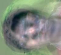
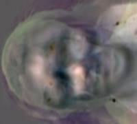
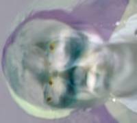
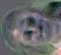
Results
The first five eigenfaces:

Now the results of the classification:
We can see that the algorithm only misclassified one point. Notice that the groups are almost linearly separable, so eigenfaces was an extremely helpful representation.
Final thoughts
A gaussian mixture model is a powerful technique for unsupervised learning. With Variational Inference, we can give more abilities to the mixture, like working with missing values, or adding additional levels to the hierarchical model. GMM are also the principles for learning advances models like Hidden Markov Models.

Comments